 Nederlandse versie
Nederlandse versie
Nederlandse versie
This document contains a Java-applet that demonstrates the central limit theorem through simulation. A user's guide is available.
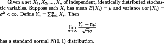
Roughly, the central limit theorem says that the sum of a number of (independent) samples taken from any distribution is approximately normally distributed. As we add more terms the approximation becomes better. This does not only apply to the sum but also to the average (which makes sense if one knows that if X has a normal distribution then it follows that also aX has a normal distribution). In mathematical terms:
This theorem explains why we might see so many times a normal distribution in practice: a stochastic variable that is influenced by a large number of independent processes will be approximately normally distributed,
A sample is drawn from a user specified distribution. In general you will need to add more terms to achieve a normal-like distribution if you choose a "wild" distribution. E.g. for a "reasonable" distribution we get the following pictures:
| distribution | summation length=2 | summation length=5 | summation length=10 |
|---|---|---|---|
 |
 |
 |
 |
When we add just 5 terms, the summation is already quite normal. If we choose however a real wild distribution, things look differently:
| distribution | summation length=2 | summation length=5 | summation length=10 |
|---|---|---|---|
 |
 |
 |
 |
Only after adding about 10 terms we start to see a bell-curve
.
In the second window the cumulative distribution function is shown. It is kept in sync with the density that you specify. The inverse of this function is used to draw samples.
The upper-right window allows you to set several parameters. Notice that it is important that the simulation length is much larger than the summation length. If we draw just 1000 observations, and have a summation length of 100 then only 10 observations are available for the sum.
The windows at the bottom show the resulting distributions of three different summations. When using a summation length of 1, the empirical distribution should be very much like the one you specified. The large the summation length the more the empirical distributions will look like a normal distribution.
The Java source of this applet can be downloaded and copied.
The idea of moving the control points came from a Java applet by Michael Heinrichs (Curve).
The mathematical formulation is rendered as a GIF file using Latex and textogif. We used workstations from GAMS Development Corp, Washington DC for this.
The screen shots were produced by snap32.
The Java applet is developed using Symantec's Cafe.